Sparse neural networks have garnered attention due to their theoretical promise of lowered computational demands and memory savings. However, to this date, the theoretical gains have largely failed to materialize due to the lack of hardware support for this kind of models. In this work, we explore the idea of neuron recycling which is inspired by pruning - a method often employed to induce sparsity in neural networks. We also present lessons we have learned along the way.
Introduction
Pruning is a well-established technique used to sparsify neural networks (LeCun et al., 1989; Han et al., 2015). It relies on the fact that typically a large part of a trained neural network can be masked without impacting the accuracy of the network, albeit often requiring additional fine-tuning in order to regain some lost performance. Despite multiple works proposing various neuron-selection criteria for pruning, magnitude-based pruning remains a viable option. The Lottery Ticket Hypothesis (Frankle and Carbin, 2019) is a major finding on the way to explain how the initialization impacts neural networks. The main point of the LTH is that through iterative pruning, performant subnetworks depending on the initialization can be found in neural networks. Those well-initialized network fragments are the namesake of LTH (the “lottery tickets”). Although some notions of the original LTH paper have been challenged (Frankle et al., 2020), it has remained the subject of active research and a motivation for our work.
By combining the two ideas (pruning and LTH) we arrive at a new potential technique for raising neural network performance. If we are able to remove parts of the network without hurting the performance (pruning) and the fitness of a part of a network is determined at initialization, perhaps we could re-initialize the unnecessary network parts (i. e. draw more “lottery tickets”), leading to a better-performing network.
Preliminaries
Before we move to the presentation of our experiments and findings, let’s first discuss the training setup, define key terminology, and go over the basics.
Model and training setup
In our project, we are focusing on the Transformer (Vaswani et al., 2017), since it’s a major architecture across different domains (Touvron et al., 2023; Dosovitskiy et al., 2021). For the specific type of the model, we are working on encoder-only BERT (Devlin et al., 2019). Taking into consideration available computational resources and expected iteration time (we wanted to try as many options as possible), we decided to opt for the BERT Medium configuration (with \(d_\text{model}=512\) and \(8\) attention heads). We focus on the feed-forward layer, because it is the most computationally demanding part of commonly-used transformer models and, in large models, it contains the majority of the parameters. At the same time, the amount of research focusing on the attention mechanism is overwhelming, suggesting that the feed-forward layer is a relatively unexplored area.
We trained the model for \(80{,}000\) steps (around compute-optimal number of train samples for this size of model) , with Adam (Kingma and Ba, 2017), using batch size of \(256\) and learning rate of \(0.001\). We used Kaiming uniform (He et al., 2015) initialization in the feed-forward layer. For the training objective, we use masked language modeling loss, as described in (Devlin et al., 2019).
In the following part of this post, we will often use the terms neuron and magnitude. Below are the definitions we employ.
Neuron. In the Transformer, feed-forward layer consists of two linear layers, with a nonlinearity in between. The first layer maps the input vector from \(d_\text{model}\) to \(d_\text{ff}\) dimension, and the second one from \(d_\text{ff}\) back to \(d_\text{model}\). Typically, \(d_\text{ff}\) is four times greater than \(d_\text{model}\). By neuron, we will understand all weights interacting with a particular coordinate in the \(\mathbb{R}^{d_\text{ff}}\) activation vector. In the torch implementation, a neuron’s weights are the parameters in a given row of the first feed-forward matrix and in the corresponding column in the second one.
Magnitude. To calculate magnitude of a weight, we will use its absolute value. As the magnitude of the \(i\)-th neuron we will use value of the expression \[M= \lVert x_i^{in}\rVert \cdot \lVert x_i^{out}\rVert,\] where:
- \(\lVert x_i^{in}\rVert\) - \(l_2\) norm of the \(i\)-th row in the weight matrix of the input linear layer
- \(\lVert x_i^{out}\rVert\) - \(l_2\) norm of the \(i\)-th column in the weight matrix of the output linear layer.
Pruning
Pruning is a technique used to induce sparsity and decrease the parameter count in a neural network. In simple terms, it means deleting the least important neurons (structured pruning) or weights (unstructured pruning). A typical implementation realizes this by either multiplying the output of the deleted neurons by 0 or setting the weights of the neuron to 0. A widely-used proxy for the importance of a neuron or weight is its magnitude. Notably, the network can still be trained even if the architecture doesn’t contain feed-forward layer, because the model can learn to represent the same trainsformation using only Attention. However, without FF the training time needed to achieve the same performance is much longer.
Below we present a plot with loss curves of the model gradually pruned at the FF layer, starting in step \(10{,}000\), such that the layer is completely masked in the end of the training. In this case, we perform structured pruning, i.e. we mask the whole neurons. As a comparison, we also add regular model and the one without feed-forward layer.
Interestingly, the effect of pruning can’t be visible for a significant fraction of the training time. It’s also worth noting that in the end the model without FF Layer performs slightly better than the pruned one. This is because in the first case, Attention was trained to adjust from the very beginning of the training.
The goal
The end-goal of the project was to create a method that would allow us to make better use of the parameters in the feed-forward layer. In this context, a natural question arises - against what baseline should our results be compared? To answer this question, we trained the model with differing dimensionalities of the feed-forward layer. The results are presented below.
The true BERT Medium configuration has \(d_\text{ff}=2048\). As we might expect, the performance drops when \(d_\text{ff}\) is decreased and improves when \(d_\text{ff}\) is increased. In particular, the model with the feed-forward layer two times wider than the baseline achives the same loss in approximately 20% fewer steps. This shows the direction for our project: through neuron recycling, we want the model to behave more like the one with larger \(d_\text{ff}\) by making a better use of available parameters.
Understanding neuron magnitudes
One of the key inspirations for our work was structured pruning, where neuron/filter magnitude is often chosen as the measure of significance (Li et al., 2017; He et al., 2018). We were interested in how this metric evolves during the training process. At first, we thought a histogram of neuron magnitudes would exhibit a normal distribution. However, our experiments showed something different. The following graph shows evolution of neuron magnitudes throughout the training process.
In the early stages of training, the neurons split into two groups, one with much lower magnitudes than the other. This finding opens up many discussion topics. One could guess that the neurons belonging to the group with smaller magnitudes potentially don’t hold much importance and can be pruned freely. However, it’s also possible that these neurons, though small, play a critical role in specific tasks.
This phenomenon is not limited to the first layer of the network. We have observed it in all layers, apart from the last one, as shown in the following plot.
After examining these experiments, we were trying to understand why in the early layers we observed two distinct groups of neurons, categorized by their magnitudes. One possible explanation is that certain parts of the network receive a smaller signal and are slower to improve in training. We designed an experiment to check that. We periodically froze all parts of the network except for the feed-forward component and continued to train it for several batches of data. We hypothesized that in this scenario, weaker neurons might catch up, resulting in a more even distribution. We called this procedure overtraining feed-forward layer. It’s important to note that this approach is impractical and computationally heavy, but we wanted to use it for the purpose of illustration. The results are depicted in the following plot.
We can see that the group of weaker neurons has moved to the right after performing additional training of the FF part. However, neurons still form two distinct groups: overtraining the whole layer is not enough for the weaker ones to catch up. In the next experiment, we have examined the scenario of retraining only small magnitude neurons, only large magnitude neurons and random subsets. How does it affect the performance? The results are depicted on the following plot.
Overtraining only the smallest neurons yields the best results when compared to reinforcing high-magnitude ones. Notably, overtraining the small ones gives similar gains in performance to working on the entire layer! Contrarily, ampifying the highest ones gives gains comparable to no overtraining at all. This provides a compelling argument in favor of our technique, suggesting that we can achieve significant gain by improving the the functionality of low-magnitude neurons.
Magnitudes in openly available pretrained models
So far, we have performed a series of experiments in one particular setting. We were curious to see how our observations would translate to well-established, large-scale foundation models like BERT Large or T5.
There is a clear difference between the plots above. Magnitudes in T5 seem similar to those in our smaller models, while BERT Large presents a more balanced distribution. What could account for these variations? It turns out that an important difference between the training process of these models was the use of weight decay. Intuitively, adding a component to the loss function that corresponds to the magnitudes of weights, helps balance the magnitudes of neurons. In the following part of the article we will further explore the idea of explicitly changing the magnitude distribution through modification of the loss function.
Findings presented above support the idea of exploring neuron recycling and offer a good foundation for further experiments. In the next sections, we will present results on this topic and share our insights.
Recycling
The central part of our work was a method we called neuron recycling. The process consists of three phases, repeated periodically: training, selection and reinitialization.
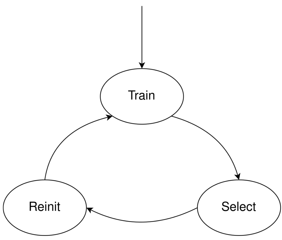
- In the training phase, the model is trained to predict masked tokens (masked language modelling).
- In the selection phase, the least important neurons are determined, where the baseline criterion is neuron magnitude.
- In the reinitialization phase, new weights are assigned to neurons.
Although this procedure is conceptually simple, it allows for many degrees of freedom. Here are some choices that can be made:
- The number of training steps before consecutive selection / reinitialization phases
- The percentage of recycled neurons
- Selection / reinitialization strategies
After examining the pruning literature, we found that the simple magnitude-based approach works well in most cases (Blalock et al., 2020; Maene et al., 2021). Moreover, it is easy to implement and computationally efficient. This approach is also grounded in our experiments. Below we present the training curves for the model pruned gradually using different criterions: high/low magnitude and random neurons.
As you can see, removing low magnitude neurons hurts the model the least, and removing high magnitude ones cases the largest loss. This is a good argument that this criterion correlates well with neuron significance.
Baseline recycling
The most straightforward reinitialization scheme is to sample the weights of the reinitialized neurons from the initial distribution. After examining the performance of this solution, we could not see any difference between recycling and vanilla training.
As a sanity check, we have examined the histogram presenting the number of times each neuron was recycled, discovering that the same small subset of neurons was being reinitialized over and over during training.
As we have seen in the previous section, on average magnitude of neurons grows throughout the training. Therefore, sampling from the initial distribution will cause the reycycled neurons to have even lower magnitudes. As an effect, they are unable to catch up to before another selection phase. Thus, the recycled neurons are caught up in a vicious cycle in which they are always recycled before achieving high magnitude.
Immunity
To address the problem we observed in the previous approach, we tried another strategy - recycling with immunity. The idea here is to encourage diverse recycling by making each recycled neuron immune to further recycling for some predefined number of steps. We hypothesized that a reinitialized neuron needs some time to grow, which was not possible in the initial setting. The following plot illustrates that immunity prevents the recycled neurons from being catched in a vicious cycle.
Higher number of immunity rounds (i.e. number of selection phases when a newly recycled neuron can’t be chosen) causes more neurons to be reinitialized at least once. Unfortunately, this eventually causes well-behaving parts of the network to be chosen for recycling. As an effect, the performance drops.
Modifying reinitialization distribution
As we have pointed out before, magnitude and weight distribution drifts away from the initial distribution as the training progresses. However, during our initial attempts, we initialized the weights sampling from the initial distribution. To fix this issue, we decided to try out another weight sampling technique. In this approach we used the normal distribution with mean and standard deviation equal to the mean and standard deviation of all the weights in the respective layer. This approach, like immunity, eliminated the vicious cycle problem.
However, this process introduced a lot of noise with adverse effect on the model’s loss.
Copying existing neurons
In the problem of growing or warm starting neural networks, the aim is to gradually add new weights to the model througout the training. In the case of Large Language Models, this topic is mentioned in the Gopher (Rae et al., 2022) paper. In particular, the authors describe multiple strategies for adding new neurons to the feed-forward layer and conclude that copying existing ones (with an addition of small noise) seems to give the best results. We tried this approach in our setting, but couldn’t observe better performance.
Smooth recycling
We came up with the hypothesis that neuron recycling could actually work better if it didn’t have sudden and discrete changes in neuron values. These sharp changes plausibly destabilize the training process. This issue is clear in sudden loss spikes, such as those observed in the recycling with modified distribution part. It may be particularly problematic that the statistics of the optimizer need to adjust to the new values, but they don’t have time to do that. To make the recycling process smoother, we modified our strategy to linearly interpolate between the old weights of the neuron and the their target values. More precisely, the new value assigned for a recycled weight in this approach is \[ x = \alpha \ x_{target} + (1-\alpha) \ x_{old},\] where:
- \(x_{target}\) - target value chosen for the weight; this parameter is trainable right away
- \(x_{old}\) - old value of the weight before recycling; this value is no longer trainable
- \(\alpha\) - non-trainable parameter, changed linearly from 0 to 1 over 1000 steps following the selection phase.
With this modification, we saw that the training loss became smoother. However, the solution was still not able to beat the baseline.
Tangent - Midpoint Loss
While inspecting the distribution of neuron magnitudes during the training, we can notice that it is quite uneven - a large percentage of neurons remains small, and the distribution is right-skewed. Since the goal of our project was to reduce the number of low-quality, i.e., small neurons, we came up with a pretty risky solution: Midpoint Loss. The idea was to introduce an additional loss term that would encourage neuron growth and “even-ness” of the magnitude distribution. The general equation for the midpoint loss is
\[ Loss = \sum_{l = 1}^{L} \sum_{n = 1}^{d_\text{ff}} \ d\left( M_{l,n}, \ sg\left(\bar{M}_{l}\right) \right)\] where:
- \(M_{l,n}\) - magnitude of th \(n^{\text{th}}\) neuron in the \(l^{\text{th}}\) layer. In some experiments we used the \(log\) of the magnitude
- \(\bar{M}_{l}\) - average neuron magnitude in layer \(l\), typically calculated as arithmetic mean. In some experiments, median was used instead due to its robustness to outliers
- \(sg\) - stops the gradient from flowing through
- \(d\) - distance function, typically \(l_1\) or \(l_2\)
- \(d_\text{ff}\) - number of neurons in a layer. In some experiments, we only summed over neurons with magnitude below the average magnitude of the layer, to encourage growth of small neurons, without thwarting the growth of the large ones
- \(L\) - number of layers.
Since this idea is quite similar to weight decay, we decided not to optimize this term with Adam, but to split it from the task loss and optimize it using simple gradient descent - a similar technique is used in AdamW (Loshchilov and Hutter, 2019) to incorporate weight decay loss term.
Midpoint loss achieved the goal of boosting the small neurons, however it failed to make a positive impact on the model’s performance.
Conclusion
In this work, we described our attempts to integrate pruning and Lottery Ticket Hypothesis via neuron recycling. Although we were not able to beat the baseline using our technique, we explored the topic thoroughly and conducted a series of experiments, providing valuable insights into the inner workings of a transformer. We hope that our findings may be a helpful resource for future studies and investigations in this area.